When deep learning is used in sensitive domains such as healthcare and autonomous control, we should question not just the accuracy but also the confidence of the models being deployed. For example, we would like an autonomous vehicle to not only correctly identify the objects in it surroundings but to also provide a measure of how uncertain it is about it’s outputs - allowing for an area of uncertainty to be approached with extra caution. Research over the past few years has made progress towards efficient methods of obtaining uncertainty from deep models, and these techniques have shown some uptake in industry as well. In this article, we’ll explore the basics of bayesian deep learning, and implement a relatively recent method for recovering the uncertainty from a neural network: the Bayes by Backprop algorithm (Blundell et al. ‘15).

This article assumes familiarity with neural networks, and code is written in Python and PyTorch with a corresponding notebook. The theory covered in the first few sections here can be a bit hard to understand on first pass, so feel free to jump to the code examples further below to see implementations.

Terminology

All notation will be kept as close to that of the paper as possible. We can apply Bayes Rule onto the weights \(\mathbf{w}\) of a neural network, given data \(\mathcal{D}\):

\(\mathbf{w}\) are the weights of the model.
\(\mathcal{D}\) is the training data in the form of a set \((x_i,y_i)_i\), where \(x_i\) is an input and \(y_i\) is the correct output.
\(P(\mathbf{w} \vert \mathcal{D})\) is the posterior probability of \(\mathbf{w}\). This is a probability distribution over the weights, given an observed set of data.
\(P(\mathcal{D} \vert \mathbf{w})\) is the likelihood of \(\mathbf{w}\). Note that this is a probability distribution over the data, given a fixed setting of weights.
\(P(\mathbf{w})\) is the prior probability on \(\mathbf{w}\). This represents our initial beliefs on the distribution over the weights, before seeing any data.
\(P(\mathcal{D})\) is the evidence (also called the marginal likelihood) of the data

We will often be using logarithmic equivalents of these distributions in calculations. Calculating log-probabilities has better numerical stability when operating at small values close to \(0\) (which is where most probability values will be), since their log equivalents will be large negative values and the imprecise multiplication of these small values becomes a more stable addition of their logarithms.

Bayesian Inference and Prediction

To treat a neural network in a probabilistic manner, we represent each of it’s weights using a distribution rather than a single numeric value as is commonly used. A neural network can be viewed as a probabilistic model \(P(y \vert x, w)\). In the common case of classification, this corresponds to the softmax output of a network (i.e. probabilities over a categorical distribution).

The normal approach to training neural networks by updating weights using gradient descent seeks to find the weights which best explain the data. This can be seen as learning the weights which maximize the likelihood \(P(\mathcal{D} \vert \mathbf{w})\), through Maximum Likelihood Estimation (MLE):

This is the frequentist perspective, where the weights of our model are fixed, but the data is viewed as a random variable (even though we generally use an unchanging training set). If we instead view the data as being fixed and the model weights as being a random variable, we can train to maximize the posterior \(P(\mathbf{w} \vert \mathcal{D})\) via Maximum a Posteriori (MAP) learning. This is equivalent to the MLE objective with an additional regularization term using a prior distribution over the weights:

Having obtained the MLE or MAP weights, prediction can be viewed as simply using our model with these learned weights fixed:

Inference is the process of computing the entire posterior distribution \(P(\mathbf{w}\vert \mathcal{D})\). Doing so allows us to perform prediction by taking a weighted expectation over all possible values for \(\mathbf{w}\):

Variational Inference

Unfortunately inference and prediction as described above are generally intractable for neural networks. While the prior \(P(\mathbf{w})\) is something we can choose and the likelihood \(P(\mathcal{D}\vert\mathbf{w})\) can be computed straightforwardly given the data, the evidence \(P(\mathcal{D})\) in the denominator of the posterior is more problematic to calculate as it requires integration over the very high-dimensional space of weights and has no analytical solution:

We will need to employ approximations in order to make progress. Variational inference operates by constructing a new distribution \(q(\mathbf{w} \vert \theta)\), over the weights \(\mathbf{w}\) and parameterized by \(\theta\), that approximates the true posterior \(P(\mathbf{w} \vert \mathcal{D})\). More concretely, it finds the setting of the parameters \(\theta\) which minimizes the \(KL\)-divergence between \(q\) to \(P\).

The \(KL\)-divergence is an information-theoretic measure of the difference between distributions. Importantly, it is not a true distance metric since it is not symmetric between distributions, as its definition shows:

We substitute this into the previous equation and reformulate it to only depend on values we know:

Directly from this, we can construct a cost function which we will seek the minimum setting of \(\theta\) for:

This cost function is a balance between having a variational posterior that is close to the prior we choose, yet also able to explain the complexity of the data well.

As an aside, the negative of this cost, \(-F\) is frequently referred to as the evidence lower bound (ELBO), as it provides a lower bound to the evidence.

Thus, when we minimize our cost function, we are also maximizing the ELBO. It’s important to note here that Variational inference is known to underestimate the uncertainty of models.

Bayes by Backprop

Calculating the expectation of the likelihood over the variational posterior is computationally prohibitive, so we (once more) will rely on an approximate method to determining it. We approximate our cost function using sampled weights:

When using automatic differentiation as provided by frameworks such as PyTorch, we only need to worry about implementing this sampling, and setting up the cost function as above, and can leverage our usual backpropagation methods to train a model.

Reparameterized Gaussian

class Gaussian(object):
    def __init__(self, mu, rho):
        super().__init__()
        self.mu = mu
        self.rho = rho
        self.normal = torch.distributions.Normal(0,1)
    
    @property
    def sigma(self):
        return torch.log1p(torch.exp(self.rho))
    
    def sample(self):
        epsilon = self.normal.sample(self.rho.size())
        return self.mu + self.sigma * epsilon
    
    def log_prob(self, input):
        return (-math.log(math.sqrt(2 * math.pi))
                - torch.log(self.sigma)
                - ((input - self.mu) ** 2) / (2 * self.sigma ** 2)).sum()

Gaussian Scale Mixture Prior

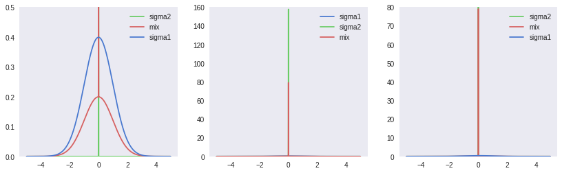
The authors suggest the use of a scaled mixture of two gaussians for the prior distribution on weights. Both gaussians are zero mean, but with separate variances. When setting \(\sigma_1 \gt \sigma_2\) and \(\sigma_2 \ll 1\), we obtain a spike-and-slab prior that combines a heavy tail (\(\sigma_1\)) with a concentration around the 0 mean (\(\sigma_2\)). Accordingly, this distribution’s probability function is as follows:

As the prior parameters are fixed and will not be modified in training, we don’t need to use a reparameterized Gaussian here:

class ScaleMixtureGaussian(object):
    def __init__(self, pi, sigma1, sigma2):
        super().__init__()
        self.pi = pi
        self.sigma1 = sigma1
        self.sigma2 = sigma2
        self.gaussian1 = torch.distributions.Normal(0,sigma1)
        self.gaussian2 = torch.distributions.Normal(0,sigma2)
    
    def log_prob(self, input):
        prob1 = torch.exp(self.gaussian1.log_prob(input))
        prob2 = torch.exp(self.gaussian2.log_prob(input))
        return (torch.log(self.pi * prob1 + (1-self.pi) * prob2)).sum()

Implementation

We now have all the components we need to construct a single bayesian network layer:

class BayesianLinear(nn.Module):
    def __init__(self, in_features, out_features):
        super().__init__()
        self.in_features = in_features
        self.out_features = out_features
        # Weight parameters
        self.weight_mu = nn.Parameter(torch.Tensor(out_features, in_features).uniform_(-0.2, 0.2))
        self.weight_rho = nn.Parameter(torch.Tensor(out_features, in_features).uniform_(-5,-4))
        self.weight = Gaussian(self.weight_mu, self.weight_rho)
        # Bias parameters
        self.bias_mu = nn.Parameter(torch.Tensor(out_features).uniform_(-0.2, 0.2))
        self.bias_rho = nn.Parameter(torch.Tensor(out_features).uniform_(-5,-4))
        self.bias = Gaussian(self.bias_mu, self.bias_rho)
        # Prior distributions
        self.weight_prior = ScaleMixtureGaussian(PI, SIGMA_1, SIGMA_2)
        self.bias_prior = ScaleMixtureGaussian(PI, SIGMA_1, SIGMA_2)
        self.log_prior = 0
        self.log_variational_posterior = 0

    def forward(self, input, sample=False, calculate_log_probs=False):
        if self.training or sample:
            weight = self.weight.sample()
            bias = self.bias.sample()
        else:
            weight = self.weight.mu
            bias = self.bias.mu
        if self.training or calculate_log_probs:
            self.log_prior = self.weight_prior.log_prob(weight) + self.bias_prior.log_prob(bias)
            self.log_variational_posterior = self.weight.log_prob(weight) + self.bias.log_prob(bias)
        else:
            self.log_prior, self.log_variational_posterior = 0, 0

        return F.linear(input, weight, bias)

And can also construct the full 2-layer fully connected neural network model:

class BayesianNetwork(nn.Module):
    def __init__(self):
        super().__init__()
        self.l1 = BayesianLinear(28*28, 400)
        self.l2 = BayesianLinear(400, 400)
        self.l3 = BayesianLinear(400, 10)
    
    def forward(self, x, sample=False):
        x = x.view(-1, 28*28)
        x = F.relu(self.l1(x, sample))
        x = F.relu(self.l2(x, sample))
        x = F.log_softmax(self.l3(x, sample), dim=1)
        return x
    
    def log_prior(self):
        return self.l1.log_prior \
               + self.l2.log_prior \
               + self.l3.log_prior
    
    def log_variational_posterior(self):
        return self.l1.log_variational_posterior \
               + self.l2.log_variational_posterior \
               + self.l2.log_variational_posterior
    
    def sample_elbo(self, input, target, samples=SAMPLES):
        outputs = torch.zeros(samples, BATCH_SIZE, CLASSES)
        log_priors = torch.zeros(samples)
        log_variational_posteriors = torch.zeros(samples)
        for i in range(samples):
            outputs[i] = self(input, sample=True)
            log_priors[i] = self.log_prior()
            log_variational_posteriors[i] = self.log_variational_posterior()
        log_prior = log_priors.mean()
        log_variational_posterior = log_variational_posteriors.mean()
        negative_log_likelihood = F.nll_loss(outputs.mean(0), target, size_average=False)
        loss = (log_variational_posterior - log_prior)/NUM_BATCHES + negative_log_likelihood
        return loss

net = BayesianNetwork()

Training

def train(net, optimizer, epoch):
    net.train()
    for batch_idx, (data, target) in enumerate(tqdm(train_loader)):
        net.zero_grad()
        loss = net.sample_elbo(data, target)
        loss.backward()
        optimizer.step()

optimizer = optim.Adam(net.parameters())
for epoch in range(TRAIN_EPOCHS):
    train(net, optimizer, epoch)

By observing the losses, we can see that optimization is able to reduce both the complexity and data loss over the training dataset:

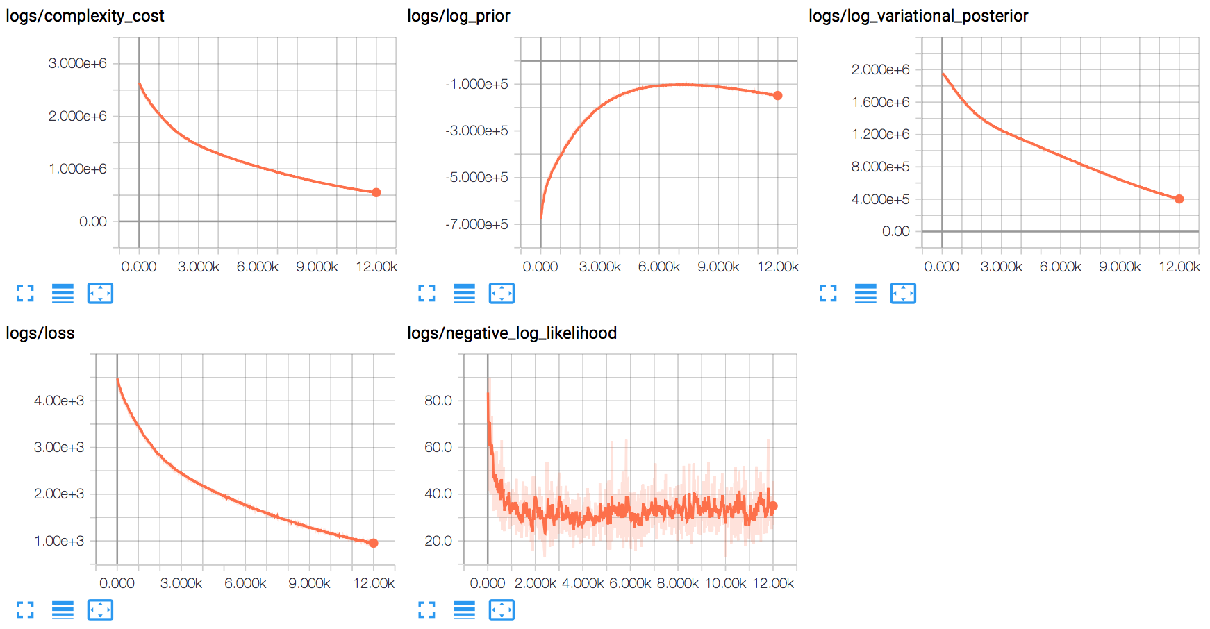
The training process appears to quickly optimize for the data component, before largely shifting to finding a good distribution around the mean weights.

Model Ensembling

Having trained distributions on the weights of our model, we now effectively have an infinite ensemble of neural networks. We can leverage this by combining the outputs from different samples of our model weights:

def test_ensemble():
    net.eval()
    correct = 0
    corrects = np.zeros(TEST_SAMPLES+1, dtype=int)
    with torch.no_grad():
        for data, target in test_loader:
            outputs = torch.zeros(TEST_SAMPLES+1, TEST_BATCH_SIZE, CLASSES)
            for i in range(TEST_SAMPLES):
                outputs[i] = net(data, sample=True)
            outputs[TEST_SAMPLES] = net(data, sample=False)
            output = outputs.mean(0)
            preds = preds = outputs.max(2, keepdim=True)[1]
            pred = output.max(1, keepdim=True)[1] # index of max log-probability
            corrects += preds.eq(target.view_as(pred)).sum(dim=1).squeeze().cpu().numpy()
            correct += pred.eq(target.view_as(pred)).sum().item()
    return corrects

Executing this function produces the following output:

Component 0 Accuracy: 8533/10000
Component 1 Accuracy: 8485/10000
Component 2 Accuracy: 8555/10000
Component 3 Accuracy: 8548/10000
Component 4 Accuracy: 8496/10000
Component 5 Accuracy: 8472/10000
Component 6 Accuracy: 8529/10000
Component 7 Accuracy: 8525/10000
Component 8 Accuracy: 8545/10000
Component 9 Accuracy: 8531/10000
Posterior Mean Accuracy: 8691/10000
Ensemble Accuracy: 8765/10000

Due to the choice of a gaussian distribution for our variational posterior, the mean weights are also the median and mode weights. We can see from these results that combining the outputs of samples of our model provides a better test accuracy than any individual sample (including that from the mean weights).

Measuring Uncertainty

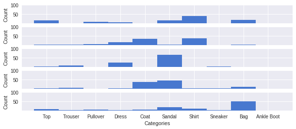
In-domain uncertainty on FMNIST

Instead of just combining the outputs of samples from our model, we can instead graph a histogram of each sample’s individual prediction. By doing so we can now visualize our model’s uncertainty on the following five entries from the FMNIST test set:

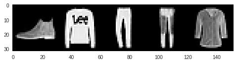
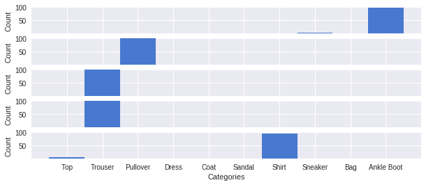
Sampling 100 times from the model, we see that it is highly confident in its overall correct predictions. The slight uncertainty for the boot and the shirt also make some sense, as a sneaker is the most similar to a boot, and a top is the most similar to a shirt.

Out-of-domain uncertainty on MNIST

Our model works well on FMNIST data, but what happens when it is exposed to data from a very different domain? We can test this by seeing what predictions the model makes for handwritten digits from the MNIST dataset:

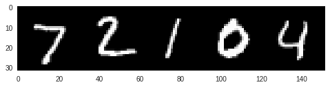
We can see here that the 100 sample predictions are far more spread out than before, and our model is not nearly as confident in any one prediction.

Closing Thoughts

While this paper really helped me learn new concepts in this field, the lack of clear information on hyperparameter selection was frustrating. As well, training proved to be very sensitive to initial values for parameters, which was not mentioned in the paper.

When the number of parameters is lower (e.g. 100 units/layer, 1 hidden layer), training tends towards less uncertainty on MNIST. I also found that initially training would improve on likelihood, before learning better weight distributions that could reflect good uncertainty on MNIST.

Additional Resources

Bayesian and Variational Inference

Intuitive Introduction to the KL Divergence
Slides on Inference
Notes on Inference

Bayes by Backprop

Tutorial and Gluon Implementation
Tutorial and TensorFlow/Edward Implementation
Alternative PyTorch Implementation